excel_course

Excel course

• Basic topics
  • Change language
  • Select a range of cells
  • Resize rows and columns
  • Auto-resize rows and columns
  • Add a new line in a cell
  • Wrap text
  • Freeze panes
  • Merge cells
  • Cell types
  • Advanced copy paste
  • Clear cells
• Formulas
  • Basic operators
• Throubleshooting
  • Having “#####” inside a cell
  • Unexpected numbers when copy-pasting dates
  • Unexpected warning “There’s already data here. Do you want to replace it?” or “This operation will cause some merged cells to unmerge”

Basic topics

Change language

Using Excel in English is a good idea because it’s easier to find help online. To change the language, go to File > Options > Language and set the Display Language to English. Then restart Excel.

Select a range of cells

In order to select all cells in the current sheet, press the small square button in the top left corner of the sheet, between the column and row headers.

💡 TIP: You can also use the keyboard shortcut Ctrl + A.

To select entire rows or columns, click on the row or column header. To select multiple rows or columns, click on the first row or column header and drag the mouse until satisfied.

To select a range of cells, click on the first cell and drag the mouse to the last cell. To select multiple ranges of cells, hold the Ctrl key while selecting the ranges.

💡 TIP: To expand or shrink the selection, press and hold the Shift key while using the arrow keys. Use Ctrl + Shift + Arrow to expand the selection to the last non-empty cell.

Resize rows and columns

To resize rows and columns, hover the mouse on their borders, then click and drag the border to the desired size.

💡 TIP: If you select multiple rows or columns and resize them, they will all be resized to the same size.

Auto-resize rows and columns

To auto-resize columns, double-click on the right border of the column header. You can also select multiple columns and double-click the border of any of them to resize all.

The same applies to rows.

Add a new line in a cell

To add a new line in a cell, simply press Alt + Enter. To facilitate writing, you can also expand the text box by pressing the arrow on the right side of it. Then drag the lower border to expand vertically.

Wrap text

If you have a long text inside a cell and you want it to be wrapped according to the cell width, you can use the Wrap Text button in the Home tab.

Freeze panes

There are 3 ways to freeze panes:

• Freeze a custom range
• Freeze the first row
• Freeze the first column

To access these options, go to View > Freeze Panes. Options are: Freeze Panes, Freeze Top Row, and Freeze First Column.

Two of the options are self-explanatory. To freeze a custom range instead, select the first cell of the sheet that you want to move. Now click on View > Freeze Panes > Freeze Panes. This will freeze all rows and columns above and to the left of the selected cell.

Once frozen, go to View > Freeze Panes again, and notice that a new option is available: Unfreeze Panes.

Merge cells

To merge cells, select the cells you want to merge and click on Home > Merge & Center. Click it again to unmerge the cells.

Cell types

There are multiple cell types, each type influences how the cell is displayed to the user. Changing the cell type never changes the value of the cell, what changes is how the value is displayed.

The main cell types are:

• General
  • This is the default cell type. It tries to guess the type of the value and display it accordingly.
• Number
  • This cell type is used to display numbers. It aligns the numbers to the right and adds a consistent number of decimal places and might add the thousands separator.
  • 💡 TIP: To change the number of decimal places, use the Increase Decimal and Decrease Decimal buttons in the Home tab.
  • 💡 TIP: Be aware that the fixed number of decimals might hide the true value of the cell because it rounds the value.
• Currency
  • This cell type is used to display currency values. It aligns numbers to the right, adds the thousands separator, and the currency symbol.
• Accounting
  • This is similar to the Currency cell type, but it also aligns the minus sign of negative numbers.
• Short Date
  • This displays the date in a short format like dd/mm/yyyy. However, the actual format depends on the language chosen in Excel.
  • 💡 TIP: Be aware that, for example, the date 21/07/2014 is internally represented via the number 41841. Therefore, when copy-pasting dates, if an unexpected number shows up, the problem is probably that the destination cell doesn’t have the correct cell type.
• Long Date
  • Same as Short Date, but the month is spelled out and the day of the week is added.
• Time
  • This displays the time in a short format like hh:mm:ss. However, the actual format depends on the language chosen in Excel.
• Percentage
  • This displays the number as a percentage, with a fixed number of decimal places and a % symbol. For example, 0.5 becomes 50%.
• Fraction
  • This displays the number as a fraction. For example, 0.5 becomes 1/2.
• Scientific
  • This displays the number in scientific notation. For example, 100000 becomes 1E+05.
• Text
  • This displays the value as text, without any formatting.
• There is also the possibility to create a custom cell type by using special format characters.

💡 TIP: Many of the above formats have a number of possible customizations. Click More Number Formats from the cell type dropdown to access them.

Advanced copy paste

When copy-pasting cells, you can choose what to paste.

To access the advanced paste menu, right-click on the cell that you want to fill.

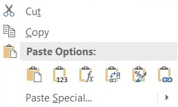
Options, going left to right, are:

• Paste
  • The default copy-paste behavior.
  • This pastes everything: formatting, values, and formulas.
  • ⚠️ ATTENTION: When pasting formulas, all the references will be relative. For more information see Formula references.
• Values
  • This pastes only the values of the cells.
  • 💡 TIP: This is useful when you want to copy-paste the result of a formula and you don’t want it to update when data changes.
• Formulas
  • This pastes only the formulas of the cells without formatting.
  • ⚠️ ATTENTION: When pasting formulas, all the references will be relative. For more information see Formula references.
• Transpose
  • This pastes the cells in a transposed way, meaning that rows become columns and columns become rows.
• Formatting
  • This pastes only the formatting of the cells.
• Link
  • This pastes an absolute reference to the copied cells.
  • This means that every time the copied cells change, the pasted cells will also change.

The Paste Special menu contains other less common options.

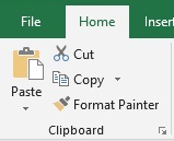
💡 TIP: To copy formatting, you can also select the source cells and click Format Painter from the Home tab. Then, select the cells to paste the formatting to.

Clear cells

To clear cells, select the cells you want to clear and click on Home > Clear. Options are:

• Clear All
  • This clears everything: formatting, values, and formulas.
• Clear Formats
  • This clears only the formatting of the cells, keeping the values and formulas.
• Clear Contents
  • This clears values and formulas.
• Clear Comments
  • This clears only the comments of the cells.
• Clear Hyperlinks
  • This clears only the hyperlinks of the cells but the text remains formatted as if it was still a hyperlink.
• Remove Hyperlinks
  • This removes the hyperlinks of the cells, returning the text to its original formatting.

Formulas

The main purpose of Excel is to perform calculations based on the data in the cells. This is done via formulas.

To create a formula, select a cell and type =. From now on, the cell will execute the formula rather than showing what you typed.

A simple example is =1+1. This formula will show 2 in the cell.

You can also reference other cells. For example, if you type =A1, the cell will show the value of the cell A1. If you type =A1+A2, the cell will show the sum of the values of the cells A1 and A2.

💡 TIP: You can also reference cells from other sheets. For example, if you type =Sheet2!A1, the cell will show the value of the cell A1 in the sheet Sheet2.

Basic operators

To operate on values, you can use the following symbols:

• + (addition)
• - (subtraction)
• * (multiplication)
• / (division)
• & (concatenation)
  • This is used to concatenate strings. For example, ="Hello" & " " & A1 might show Hello John if the value of A1 is John.
  • ⚠️ ATTENTION: When concatenating strings, you need to add the spaces manually. For example, ="Hello" & A1 will show HelloJohn.
• " (double quotes, used in pairs)
  • This is used to write text. For example, ="Hello" will show Hello.
  • In general, all the text used inside a formula needs to be enclosed in double quotes.
• = (equal)
• > (greater than)
• < (less than)
• >= (greater than or equal)
• <= (less than or equal)
• <> (not equal)
• TRUE (logical true)
• FALSE (logical false)

Operators work on specific types of values. For example, the math operators work on numbers, the & on text. Other operators such as =, >, <, and <> work on logical values and output TRUE or FALSE. For example, =2<5 outputs TRUE.

---

Throubleshooting

Having “#####” inside a cell

This happens when the cell is too short to display the value. To fix it, simply resize the cell.

Unexpected numbers when copy-pasting dates

Dates are internally represented via numbers. Therefore, when copy-pasting dates, if an unexpected number shows up, the problem is probably that the destination cell doesn’t have the correct cell type.

See also the Cell types section.

Unexpected warning “There’s already data here. Do you want to replace it?” or “This operation will cause some merged cells to unmerge”

This might happen when you try to move a range of cells partially over themselves. To avoid the error, first move the selection to an empty space and only then move it to the desired location.